IndexFiguresTables |
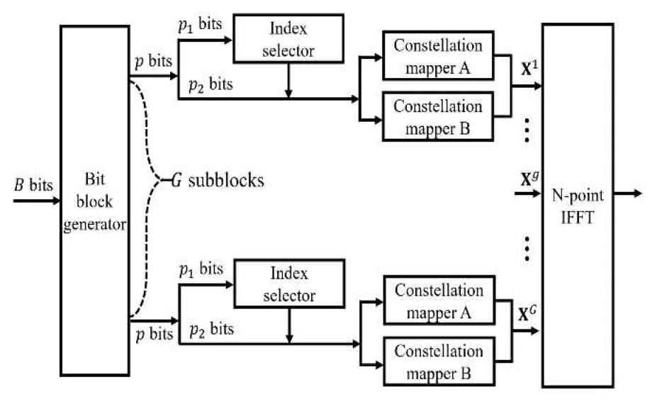
Seung-gi Choi , Kezhong Jin and Hosung ParkTwo-Layer Coding with Flexible Layer-Partitioning for Dual-Mode OFDM-IMAbstract: Dual mode orthogonal frequency division multiplexing with index modulation (DM-OFDM-IM) employs two distinguishable constellations across all subcarriers to address the low spectral efficiency of OFDM-IM. Recent studies on OFDM-IM-based systems have focused on constellation design, index pattern selection, and channel coding. A two-layer coding (TLC) scheme with successive cancellation decoding (SCD) has been proposed to improve the bit error rate (BER) of conventional OFDM-IM. However, it has not been applied to DM-OFDM-IM, and its frame error rate (FER) performance has not yet been evaluated. In this paper, we propose a method that applies TLC combined with SCD to DM-OFDM-IM. This approach addresses the challenge of DM-OFDM-IM, which faces greater difficulty in distinguishing index patterns compared to conventional OFDM-IM. We analyze the capacity of DM-OFDM-IM with TLC and demonstrate its advantage over conventional DM-OFDM-IM in terms of achievable rate. Furthermore, we propose a flexible layer-partitioning (FLP) scheme between two codewords, enabling a more flexible range of code rate variations. In addition, when decoding the second layer with SCD, only the estimated index pattern needs to be considered instead of all possible index patterns. It is shown via simulations that the proposed DM-OFDM-IM achieves a lower FER than conventional DM-OFDM-IM under various modulation parameters. Keywords: orthogonal frequency division multiplexing (OFDM) , index modulation (IM) , dual mode OFDM-IM (DM-OFDM-IM) , channel coding , two-layer coding (TLC) , flexible layer-partitioning (FLP) Ⅰ. IntroductionIndex modulation (IM) is a transmission scheme that conveys additional information by modulating the activation pattern of communication resources, and it has been the focus of extensive research in recent years[1-3]. Orthogonal frequency division multiplexing with index modulation (OFDM-IM) is a technique that groups the subcarriers of an OFDM block into subblocks, where additional information is conveyed through the activation pattern of the subcarriers[4]. OFDM-IM enhances energy efficiency by activating only a subset of subcarriers, reducing transmit power without sacrificing data rate. In addition, by conveying information through subcarrier indices, it achieves better error performance than conventional OFDM due to higher diversity orders[4]. Although OFDM-IM offers performance advantages over conventional OFDM, its spectral efficiency is inherently reduced because it utilizes only a subset of subcarriers. To address this shortcoming, dual-mode OFDM-IM (DM-OFDM-IM) was proposed, in which two distinguishable constellations are employed to modulate all subcarriers[5]. Since all subcarriers are utilized without any inactive subcarriers, the transmission rate can be significantly increased compared to OFDM-IM. Prior research in IM-related systems has focused on enhancing performance from the perspectives of constellation design, index pattern design, and channel coding. For instance, in [6] a dual-square shaped constellation was introduced, wherein symbols sharing the same mapping are positioned adjacently to facilitate dual-mode operation. An index mapping algorithm was proposed in [7] to minimize errors by ensuring that the Hamming distance between adjacent index patterns remains fixed at 2. Moreover, [8] presented a DM-OFDM-IM scheme based on a Reed– Muller codebook, which maximizes the minimum Hamming distance between index patterns. A significant challenge in OFDM-IM systems is channel decoding, as the computation of log-likelihood ratios (LLRs) becomes computationally intensive. To mitigate this issue, a low-complexity LLR calculation method for low density parity check (LDPC) decoding was introduced[9]. Furthermore, the LLR computation for symbol bits―requiring the incorporation of probabilities for all index patterns― substantially increases the computational burden. To alleviate this, a successive cancellation soft demapping approach was proposed that leverages the LLRs of the index bits during the symbol bit calculation[10]. However, the use of unreliable initial LLR estimates can adversely affect LDPC decoding, leading to degradation in frame error rate (FER). To improve reliability, subsequent studies have incorporated the concept of multi-level coding (MLC), wherein separate index and symbol codewords are generated and assigned appropriate code rates, demonstrating improved robustness against jamming attacks[11]. However, since channel coding typically achieves lower error rates with longer code lengths, the finite code lengths in practical systems limit achievable performance. To address this issue, successive cancellation decoding (SCD), which utilizes the output of index codeword decoding to aid symbol codeword decoding, was proposed along with a new radio extrinsic information transfer (NR-EXIT) algorithm[12]. However, that method is limited to OFDM-IM systems, allows for only limited code-rate variations, and does not provide FER performance results. In this paper, we propose a two-layer coding (TLC) structure for DM-OFDM-IM systems, called TLC-DM-OFDM-IM. In addition to overcoming code length limitations via SCD, the proposed scheme reduces the computational complexity of symbol bit LLR calculation. Unlike conventional DM-OFDM-IM systems that employ only bit-interleaved coded modulation (BICM), our approach incorporates the favorable properties of MLC/multi stage decoding (MSD), enabling the application of tailored code rates to each codeword and yielding significantly improved FER compared to one-layer coding (OLC) schemes. We demonstrated the theoretical advantage of TLC through capacity analysis. Nevertheless, this method is limited by inflexible code rate allocation between the two codewords, and the first layer remains relatively short. To overcome these limitations, we propose a flexible layer-partitioning (FLP) technique, in which the first layer covers the whole index bits and some of the symbol bits and the second layer covers the other part of symbol bits. This FLP technique allows for a more optimal code rate assignment within a TLC framework, as evidenced by simulation results that demonstrate superior FER performance relative to fixed code length TLC schemes. Ⅱ. Conventional DM-OFDM-IMDM-OFDM-IM divides an OFDM block into n subblocks and transmits additional bits based on the constellation pattern of each subblock. The transmitter of the DM-OFDM-IM system is illustrated in Fig. 1. First, B the information bits are divided into G subblocks. The g-th subblock contains p bit vector [TeX:] $$\mathbf{b}^{\mathrm{g}}=\left[\begin{array}{ll} \mathbf{b}_1^g & \mathbf{b}_2^g \end{array}\right],$$ which are partitioned into index bits [TeX:] $$\mathbf{b}_1^g$$ and symbol bits [TeX:] $$\mathbf{b}_2^g$$ with lengths [TeX:] $$p_1=\left\lfloor\log _2\binom{n}{k}\right\rfloor$$ and [TeX:] $$p_2=n \log _2 M,$$ respectively.
Each subblock contains n subcarriers, of which k are modulated using Constellation A [TeX:] $$\mathcal{M}_{\mathrm{A}}$$ and the remaining n-k are modulated using Constellation B [TeX:] $$\mathcal{M}_{\mathrm{B}}$$. The constellation mode of the subcarriers is determined by the index bits and the index table, such as Table 1, and the symbol bits determine the OFDM subblock [TeX:] $$\mathbf{X}^{\mathrm{g}}$$ through index pattern and the constellation pair, as illustrated in Fig. 3. The concatenated G subblocks are processed via an N-point IFFT. At the receiver, the DM-OFDM-IM system obtains symbols for all G subblocks. The received g-th subblock can be expressed as follows:
where [TeX:] $$\mathbf{H}^g=\operatorname{diag}\left(\left[H^g(1), \cdots, H^g(n)\right]\right)$$ is an n × n matrix whose diagonal elements represent the channel coefficients and we assume [TeX:] $$\mathbf{H}^g(\alpha) \sim C N(0,1) (\alpha=1, \cdots, n) . \mathbf{W}^g=\left[W^g(1), \cdots, W^g(n)\right]$$ is the additive white Gaussian noise (AWGN) vector and we assume [TeX:] $$\mathbf{W}^g(\alpha) \sim C N\left(0, N_0\right)(\alpha=1, \cdots, n)$$ In scenarios without channel coding, the receiver estimates the g-th subblock using an LLR detector[5]. Since all G subblocks are estimated in the same manner, the superscript g is omitted. First, the LLR of the [TeX:] $$\alpha \text {-th }(\alpha=1, \cdots, n)$$ subcarrier is calculated as shown in
(4)[TeX:] $$\lambda(\alpha)=\ln \left(\frac{k}{n-k}\right) \frac{\sum_{s \in \mathcal{M}_{\mathrm{A}}} \exp \left(-\frac{|Y(\alpha)-H(\alpha) s|^2}{N_0}\right)}{\sum_{s \in \mathcal{M}_{\mathrm{B}}} \exp \left(-\frac{|Y(\alpha)-H(\alpha) s|^2}{N_0}\right)} .$$The estimated index pattern
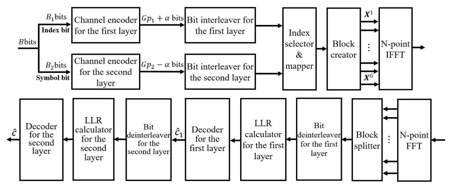
(5)[TeX:] $$\widehat{\mathfrak{B}}=\underset{b \in \mathfrak{B}}{\operatorname{argmax}} \sum_{\alpha=1}^n(-1)^{1-p(j)} \lambda(\alpha)$$is then obtained by considering all possible index patterns. Finally, the n symbols of the subblock are estimated using [TeX:] $$\mathfrak{B}.$$ Ⅲ. Proposed TLC-DM-OFDM-IM3.1 DescriptionsIn index modulation techniques, index bits determine the constellation by which the symbol bits are modulated, while the symbol bits are directly mapped onto signal points within the selected constellation. As a result, index bits and symbol bits follow different probability distributions and exhibit different error rate. Consequently, different code rates are applied to the index bits and symbol bits via TLC. Fig. 2 illustrates the block diagram of the transmitter and receiver for TLC-DM-OFDM-IM. The B message bits are divided into a first layer message bit sequence of length [TeX:] $$B_1$$ and a second layer message bit sequence of length [TeX:] $$B_2.$$ Each bit sequence is encoded with code rates [TeX:] $$R_1 \text { and } R_2,$$ respectively, yielding a first layer codeword of length [TeX:] $$E_1=G p_1$$ and a second layer codeword of length [TeX:] $$E_2=G p_2$$. The first layer consists solely of index code bits, while the second layer consists solely of symbol code bits. The signal is then transmitted in the same manner as in DM-OFDM-IM. At the receiver, decoding begins with the first layer, and the resulting output is used to decode the second layer. For first layer decoding, the LLR value for an index bit is calculated from the [TeX:] $$\mathbf{Y}^g .$$ For simplicity in the following equations, the superscript g is omitted. The LLR value of the i-th index bit is denoted by
(6)[TeX:] $$\lambda_{\mathrm{I}}(i)=\ln \frac{p\left(b_1(i)=0 \mid \mathbf{Y}\right)}{p\left(b_1(i)=1 \mid \mathbf{Y}\right)}\left(i=1, \cdots, p_1\right) .$$[TeX:] $$p\left(b_1(i)=x \mid Y\right)$$ where the i-th index bit is x can be arranged based on Bayes’ rule, as shown in
(7)[TeX:] $$p\left(b_1(i)=x \mid Y\right)=\frac{1}{2^{p_1-1} p(\mathbf{Y})} \sum_{\mathfrak{B} \in \mathfrak{B}_{i, x}} \prod_{j=1}^n p(\mathbf{Y}(j) \mid \mathfrak{B})$$When the j-th subcarrier is modulated by Constellation A [TeX:] $$\mathcal{M}_{\mathrm{A}}, p(Y(j) \mid \mathfrak{B})$$ is equal to
(8)[TeX:] $$p(Y(j) \mid \mathfrak{B})=\frac{1}{M} \sum_{s \in \mathcal{M}_A} \frac{1}{\pi N_0} \exp \left(-\frac{|\mathbf{Y}(j)-\mathbf{H}(j) s|^2}{N_0}\right)$$As in conventional DM-OFDM-IM, the LLR value of the symbol bits is calculated by considering all possible patterns, as shown in
(9)[TeX:] $$\lambda_{\mathrm{S}}(i)=\ln \frac{p\left(b_2(i)=0 \mid \mathrm{Y}\right)}{p\left(b_2(i)=1 \mid \mathrm{Y}\right)}\left(i=1, \cdots, p_2\right) .$$[TeX:] $$p\left(b_2(i)=x \mid \mathbf{Y}\right)$$ where the i-th symbol bit is x can be arranged based on Bayes’ rule, as shown in
(10)[TeX:] $$\begin{gathered} p\left(b_2(i)=x \mid \mathbf{Y}\right) \\ =\frac{1}{2^{p_1+1} p(\mathbf{Y})} \sum_{\mathfrak{B} \in \boldsymbol{\mathfrak{B}}_{i, x}} \prod_{j=1}^n p\left(\mathbf{Y}(j) \mid \mathfrak{B}, b_2(i)=x\right) . \end{gathered}$$[TeX:] $$p\left(\mathbf{Y}(j) \mid \mathfrak{B}, b_2(i)=x\right)$$ is given by
(11)[TeX:] $$\begin{gathered} p\left(\mathbf{Y}(j) \mid \mathfrak{B}, b_2(i)=x\right) \\ =\sum_{s \in \Psi_{j, i, x}} \frac{1}{\pi N_0} \exp \left(-\frac{|\mathbf{Y}(j)-\mathbf{H}(j) s|^2}{N_0}\right) \end{gathered}$$where
(12)[TeX:] $$\Psi_{\mathrm{j}, \mathrm{i}, \mathrm{x}}=\left\{\begin{array}{lll} \mathcal{M}_{i, x} & \text { if } & j=\left\lfloor\left(i+\log _2 M-1 / \log _2 M\right)\right\rfloor \\ \mathcal{M} & \text { if } & j \neq\left\lfloor\left(i+\log _2 M-1 / \log _2 M\right)\right\rfloor \end{array} .\right.$$[TeX:] $$\mathcal{M}_{i, x}$$ is the set of constellation points corresponding to the i-th index bit when it is x. And when the j-th subcarrier is modulated with Constellation A, [TeX:] $$\mathcal{M}=\mathcal{M}_{\mathrm{A}},$$ and when it is modulated with Constellation B, [TeX:] $$\mathcal{M}=\mathcal{M}_{\mathrm{B}}.$$ However, in TLC-DM-OFDM-IM, since SCD is performed, the LLR of the symbol bits is calculated by considering only [TeX:] $$\hat{\mathbf{c}}_1 .$$ If the index pattern is determined to be [TeX:] $$\mathfrak{B}_1$$ through first layer decoding, then [TeX:] $$p\left(b_2(i)=x \mid \mathbf{Y}\right)$$ in (9) is given as follows:
(13)[TeX:] $$\begin{gathered} p\left(b_2(i)=x \mid \mathbf{Y}\right) \\ =\frac{1}{2^{p_1+1} p(\mathbf{Y})} \prod_{j=1}^n p\left(\mathbf{Y}(j) \mid \mathfrak{B}_1, b_2(i)=x\right) . \end{gathered}$$In (10), the LLR for the symbol bits is calculated by considering all index patterns; however, in the TLC-DM-OFDM-IM system, only the pattern estimated from the first layer is considered. The second layer is decoded using the LLR values of the symbol bits to obtain [TeX:] $$\hat{\mathbf{c}}_2.$$ When comparing the symbol bit LLR calculation complexity of conventional DM-OFDM-IM and TLC-DM-OFDM-IM, the conventional scheme requires probability computations over all possible index patterns, resulting in a complexity of [TeX:] $$\mathcal{O}\left(p_1 n M\right) .$$ In contrast, TLC-DM-OFDM-IM adopts a successive cancellation decoding method that considers only the index pattern determined in the first codeword decoding, leading to a reduced complexity of [TeX:] $$\mathcal{O}(n M),$$ which remains constant even as the number of patterns increases. The proposed two-layer coding scheme requires two sets of encoders and decoders instead of one, which doubles the required hardware space for encoding and decoding. Additionally, since the output of the first decoder must be passed to the second decoder, a slight processing delay may occur. However, this impact is negligible, and the benefits of reduced complexity and improved performance obtained through the application of two-layer coding outweigh these drawbacks. 3.2 Capacity AnalysisTo demonstrate the effectiveness of TLC-DM-OFDM-IM, we compare the BICM capacity of TLC-DM-OFDM-IM [TeX:] $$C_{\mathrm{TLC}}$$ and conventional DM-OFDM-IM [TeX:] $$C_{\text {conv }} .$$ These BICM capacities are
(14)[TeX:] $$\boldsymbol{C}_{\mathrm{TLC}}=\frac{1}{p} \sum_{i=1}^p \mathrm{I}(b(i) ; \mathbf{Y} \mid \mathbf{I} \in \boldsymbol{\mathfrak{B}}),$$
(15)[TeX:] $$\begin{aligned} \boldsymbol{C}_{\text {conv }}=\frac{1}{p}\left\{\sum_{i=1}^{p_1} \mathrm{I}(b(i) ; \mathbf{Y} \mid \mathbf{I} \in \boldsymbol{\mathfrak{B}})\right. \\ \left.+\sum_{i=p_1+1}^p \mathrm{I}(b(i) ; \mathbf{Y} \mid \hat{\mathbf{I}})\right\} \end{aligned}$$where I is the index pattern determined by the index bits. The BICM capacity of TLC-DM-OFDM-IM should always be greater than that of DM-OFDM-IM, as given in
(16)[TeX:] $$\begin{aligned} \frac{1}{p} \sum_{i=1}^p \mathrm{I}(b(i) ; \mathbf{Y} \mid \mathbf{I} \in \mathfrak{B}) & \lt \frac{1}{p}\left\{\sum_{i=1}^{p_1} \mathrm{I}(b(i) ; \mathbf{Y} \mid \mathbf{I} \in \mathfrak{B})\right. \\ & \left.+\sum_{i=p_1+1}^p \mathrm{I}(b(i) ; \mathbf{Y} \mid \hat{\mathbf{I}})\right\} \\ \sum_{i=p_1+1}^p \mathrm{I}(b(i) ; \mathbf{Y} \mid \mathbf{I} \in \mathfrak{B}) & \lt \sum_{i=p_1+1}^p \mathrm{I}(b(i) ; \mathbf{Y} \mid \hat{\mathbf{I}}) . \end{aligned}$$Let us consider the case n = 4, k = 2 in Table 1 and M = 4 using constellation pair in Fig. 3. Also, we consider the capacity of the first bit on the first subcarrier, assuming [TeX:] $$\mathbf{I}=\mathfrak{B}_1 .$$ According to the considered case and using average entropy, the left-hand side of (16) can yield
(17)[TeX:] $$\begin{aligned} & \mathrm{I}\left(b_2(i) ; \mathbf{Y} \mid \mathbf{I} \in \boldsymbol{\mathfrak{B}}\right) \\ = & \mathrm{H}(\mathbf{Y}(1) \mid \mathbf{I} \in \boldsymbol{\mathfrak{B}})-\mathrm{H}\left(\mathbf{Y}(1) \mid b_2(1), \mathbf{I} \in \boldsymbol{\mathfrak{B}}\right) \\ = & \mathrm{H}(\mathbf{Y}(1) \mid \mathbf{I} \in \boldsymbol{\mathfrak{B}})-\frac{1}{4}\left\{\mathrm{H}\left(\mathbf{Y}(1) \mid b_2(1), \mathbf{I}=\mathfrak{B}_1\right)\right. \\ & +\mathrm{H}\left(\mathbf{Y}(1) \mid b_2(1), \mathbf{I}=\mathfrak{B}_2\right)+\mathrm{H}\left(\mathbf{Y}(1) \mid b_2(1), \mathbf{I}=\mathfrak{B}_3\right) \\ & \left.+\mathrm{H}\left(\mathbf{Y}(1) \mid b_2(1), \mathbf{I}=\mathfrak{B}_4\right)\right\} . \end{aligned}$$Since we are considering the first subcarrier, [TeX:] $$\mathbf{I}=\mathfrak{B}_1$$ can be replaced with I(1) = 1, and (17) can be arranged as denoted by
(18)[TeX:] $$\begin{gathered} \mathrm{H}(\mathbf{Y}(1) \mid \mathbf{I} \in \boldsymbol{\mathfrak{B}})-\frac{1}{4}\left\{\mathrm{H}\left(\mathbf{Y}(1) \mid b_2(1), \mathbf{I}(1)=1\right)\right. \\ +\mathrm{H}\left(\mathbf{Y}(1) \mid b_2(1), \mathbf{I}(1)=0\right)+\mathrm{H}\left(\mathbf{Y}(1) \mid b_2(1), \mathbf{I}(1)=1\right) \\ \left.+\mathrm{H}\left(\mathbf{Y}(1) \mid b_2(1), \mathbf{I}(1)=0\right)\right\} \\ =\mathrm{H}(\mathbf{Y}(1) \mid \mathbf{I} \in \boldsymbol{\mathfrak{B}})-\frac{1}{2}\left\{\mathrm{H}\left(\mathbf{Y}(1) \mid b_2(1), \mathbf{I}(1)=1\right)\right. \\ \left.+\mathrm{H}\left(\mathbf{Y}(1) \mid b_2(1), \mathbf{I}(1)=0\right)\right\} \\ =\frac{1}{2}\{\mathrm{H}(\mathbf{Y}(1) \mid \mathbf{I}(1)=1)+\mathrm{H}(\mathbf{Y}(1) \mid \mathbf{I}(1)=0)\} \\ -\frac{1}{2}\left\{\mathrm{H}\left(\mathbf{Y}(1) \mid b_2(1), \mathbf{I}(1)=1\right)+\mathrm{H}\left(\mathbf{Y}(1) \mid b_2(1), \mathbf{I}(1)=0\right)\right\} \end{gathered}$$The right-hand side of (16) can also be modified Fig. 3. Dual square QAM based constellation pair [TeX:] $$\mathcal{M}_{\mathrm{A}} \text{ and } \mathcal{M}_{\mathrm{B}}$$ for M = 4 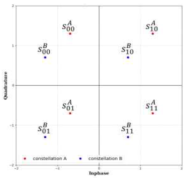 Table 1. The index table for n=4 and k=2.
to fit the considered case, in a manner similar to (18), as follows:
(19)[TeX:] $$\begin{aligned} & \mathrm{I}\left(b_2(1) ; \mathbf{Y}(1) \mid \hat{\mathbf{I}}=\mathfrak{B}_1\right) \\ & =\mathrm{H}(\mathbf{Y}(1) \mid \mathbf{I}(1)=1)-\mathrm{H}\left(\mathbf{Y}(1) \mid b_2(1), \mathbf{I}(1)=1\right) . \end{aligned}$$(16) can be expressed as (18) < (19) and rearranged as
(20)[TeX:] $$\begin{aligned} & \mathrm{H}(\mathbf{Y}(1) \mid \mathbf{I}(1)=0)-\mathrm{H}\left(\mathbf{Y}(1) \mid b_2(1), \mathbf{I}(1)=0\right) \\ & \quad \lt \mathrm{H}(\mathbf{Y}(1) \mid \mathbf{I}(1)=1)-\mathrm{H}\left(\mathbf{Y}(1) \mid b_2(1), \mathbf{I}(1)=1\right) . \end{aligned}$$[TeX:] $$\mathrm{H}\left(\mathbf{Y}(1) \mid b_2(1), \mathrm{I}(1)=1\right)$$ can be simplified as the average entropy calculation over first symbol bit [TeX:] $$b_2(1)$$ and first symbol of subblock X(1) and expressed as
(21)[TeX:] $$\begin{gathered} \mathrm{H}\left(\mathbf{Y}(1) \mid b_2(1), \mathbf{I}(1)=1\right) \\ =\frac{1}{2} \mathrm{H}\left(\mathbf{Y}(1) \mid b_2(1)=0, \mathbf{I}(1)=1\right) \\ +\frac{1}{2} \mathrm{H}\left(\mathbf{Y}(1) \mid b_2(1)=1, \mathbf{I}(1)=1\right) \\ =\frac{1}{2}\left\{\frac{1}{4} \mathrm{H}\left(\mathbf{Y}(1) \mid b_2(1)=0, \mathbf{X}(1)=\mathrm{s}_{00}^{\mathrm{A}}\right)\right. \\ +\frac{1}{4} \mathrm{H}\left(\mathbf{Y}(1) \mid b_2(1)=0, \mathbf{X}(1)=\mathrm{s}_{01}^{\mathrm{A}}\right) \\ +\frac{1}{4} \mathrm{H}\left(\mathbf{Y}(1) \mid b_2(1)=0, \mathbf{X}(1)=\mathrm{s}_{10}^{\mathrm{A}}\right) \\ \left.+\frac{1}{4} \mathrm{H}\left(\mathbf{Y}(1) \mid b_2(1)=0, \mathbf{X}(1)=\mathrm{s}_{11}^{\mathrm{A}}\right)\right\} \\ +\frac{1}{2}\left\{\frac{1}{4} \mathrm{H}\left(\mathbf{Y}(1) \mid b_2(1)=1, \mathbf{X}(1)=\mathrm{s}_{00}^{\mathrm{A}}\right)\right. \\ +\frac{1}{4} \mathrm{H}\left(\mathbf{Y}(1) \mid b_2(1)=1, \mathbf{X}(1)=\mathrm{s}_{01}^{\mathrm{A}}\right) \\ +\frac{1}{4} \mathrm{H}\left(\mathbf{Y}(1) \mid b_2(1)=1, \mathbf{X}(1)=\mathrm{s}_{10}^{\mathrm{A}}\right)+ \\ \left.\frac{1}{4} \mathrm{H}\left(\mathbf{Y}(1) \mid b_2(1)=1, \mathbf{X}(1)=\mathrm{s}_{11}^{\mathrm{A}}\right)\right\} . \end{gathered}$$For example, since [TeX:] $$\mathrm{P}\left(\left(b_2(1)=0\right) \cap\left(\mathbf{X}(1)=\mathrm{s}_{10}^{\mathrm{A}}\right)\right)=0,$$ any expression containing these terms can be eliminated. Furthermore, with the condition on I(1)=1 only, (21) can be simplified to
(22)[TeX:] $$\begin{gathered} =\frac{1}{2}\left\{\frac{1}{4} H\left(\mathbf{Y}(1) \mid \mathbf{X}(1)=s_{00}^{\mathrm{A}}\right)+\frac{1}{4} H\left(\mathbf{Y}(1) \mid \mathbf{X}(1)=s_{01}^{\mathrm{A}}\right)\right. \\ +\frac{1}{4} H\left(\mathbf{Y}(1) \mid \mathbf{X}(1)=s_{10}^{\mathrm{A}}\right) \\ \left.+\frac{1}{4} H\left(\mathbf{Y}(1) \mid \mathbf{X}(1)=s_{11}^{\mathrm{A}}\right)\right\} \\ =\frac{1}{2} H(\mathbf{Y}(1) \mid \mathbf{I}(1)=1) . \end{gathered}$$[TeX:] $$\mathrm{H}\left(\mathbf{Y}(1) \mid b_2(1), \mathbf{I}(1)=0\right)$$ in (20) is also simplified in the same manner as in (21) and (22) and substituted into (20). Consequently, (20) is as follows:
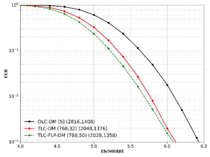
(23)[TeX:] $$\mathrm{H}(\mathbf{Y}(1) \mid \mathbf{I}(1)=0) \lt \mathrm{H}(\mathbf{Y}(1) \mid \mathbf{I}(1)=1) .$$Since Y(1) is modulated by [TeX:] $$\mathcal{M}_{\mathrm{A}},$$ the entropy of Y(1) is greater under I(1) = 1 than under I(1) = 0. Consequently, (16) holds. Similarly, the same results can be obtained for other index patterns and subcarriers through this process. 3.3 TLC-DM-OFDM-IM with FLPIn TLC-DM-OFDM-IM, the lengths of the first and second layer codewords are fixed, which limits the possible combinations of code rates. Therefore, we propose a FLP technique, called TLC-FLP-DM-OFDM-IM, which enables the adjustment of codeword lengths. Since the first layer codeword has a shorter length than the second layer codeword, the first layer covers not only the index bits but also some of the symbol bits. The message bits are divided into [TeX:] $$B_1 \text { and } B_2 .$$ For flexible layer construction, the first layer additionally covers α symbol bits. Then, the code rates for each codeword are determined. As a result, codewords of lengths [TeX:] $$G p_1+\alpha$$ and [TeX:] $$G p_2+\alpha$$ are generated through each channel encoder. Thus, by adjusting [TeX:] $$B_1 \text { and } \alpha,$$ the diversity of code rates is increased. The receiver estimates [TeX:] $$\mathrm{c}_1 \text { and } \mathrm{c}_2$$ using the same method as in TLC-DM-OFDM-IM. However, for the reallocated bits, the LLR values follow equation (9). Ⅳ. Simulation ResultsTo evaluate the performance of TLC with/without FLP for DM-OFDM-IM system, we compare the FER of conventional DM-OFDM-IM[5], and the proposed TLC-(FLP-)DM-OFDM-IM system. In DM-OFDM-IM, dual square QAM (DSQAM) based constellation pair[6] was used. We consider the Rayleigh fading channel and the channel coefficients are assumed perfectly known at the receiver. We use LDPC codes for encoding, employing the low-complexity decoding method described in [9]. [TeX:] $$R_1 \text { and } R_2$$ were determined through exhaustive search on a 2-bit basis. Henceforth, conventional DM-OFDM-IM is referred to as OLC-DM, TLC-DM-OFDM-IM is referred to as TLC-DM, and TLC-FLP-DM-OFDM-IM is referred to as TLC-FLP-DM. Fig. 4 shows the overall FER performance for N = 1024, n = 4, k = 2, M = 16 and R = 0.6. OLC-DM uses (4608, 2765) LDPC codes and TLC-DM uses (512, 70) and (4096, 2695) LDPC codes. TLC-DM uses separate codewords, resulting in a shorter code length than OLC-DM. However, due to SCD, the second layer codeword is decoded based on a more accurate index pattern, leading to improved FER performance. Furthermore, since it is unnecessary to consider all patterns when calculating the LLR for the symbol bits, it exhibits significantly lower complexity than OLC-DM. Fig. 4. Overall FER comparison of TLC-DM-OFDM-IM and OLC-DM-OFDM-IM for N = 1024, n = 4, k = 2, M = 16 and R = 0.6. 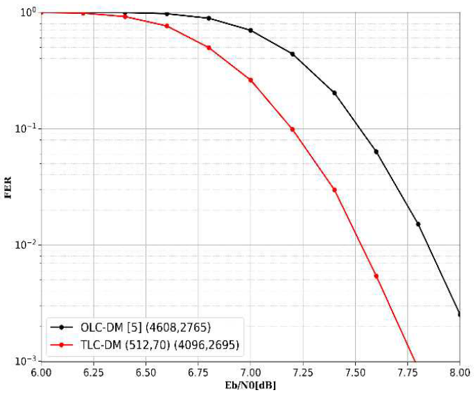 Table 2. Simulation time for symbol bit LLR calculation of TLC-DM-OFDM-IM and OLC-DM-OFDM-IM for [TeX:] $$p_1=$$ 2, 4, and 6.
To demonstrate the low-complexity decoding of TLC-DM-OFDM-IM, the simulation time required for symbol bit LLR calculation was measured, as presented in Table 2. The simulation was performed on a system with an Intel Core i7 processor at 2.9GHz and 64GB RAM. OLC-DM-OFDM-IM requires computing the probabilities of [TeX:] $$2^{p_1}$$ index patterns to calculate the LLR of symbol bits. In contrast, TLC-DM-OFDM-IM leverages the decoding result of the first layer, allowing it to consider only a single pattern when calculating the symbol bit LLR. While the simulation time of OLC-DM-OFDM-IM increases exponentially with [TeX:] $$p_1$$, TLC-DM-OFDM-IM exhibits a linear increase with n. This demonstrates the remarkable computational efficiency of TLC-DM-OFDM-IM for larger [TeX:] $$p_1$$. Fig. 5 shows the overall FER performance for N = 1024, n = 8, k = 2, M = 16 and R = 0.6. OLC-DM uses (4608, 2765) LDPC codes, TLC-DM uses (512, 4) and (4096, 2761) LDPC codes and TLC-FLP-DM uses (528, 26) and (4080, 2739) LDPC codes. Although the [TeX:] $$R_2$$ in TLC-DM is approximately 0.07 higher than the R in OLC-DM, the use of accurately decoded index bits via SCD results in a lower FER than that of OLC-DM. Furthermore, by performing FLP on the second codeword corresponding to the [TeX:] $$E_1$$ bits, a broader range of code rates can be applied to the first codeword. Consequently, TLC-FLP-DM achieves a slight improvement in FER compared to TLC-DM. Fig. 5. Overall FER comparison of TLC-(FLP-)DM-OFDMIM and OLC-DM-OFDM-IM for N = 1024, n = 8, k = 2, M = 16 and R = 0.6. 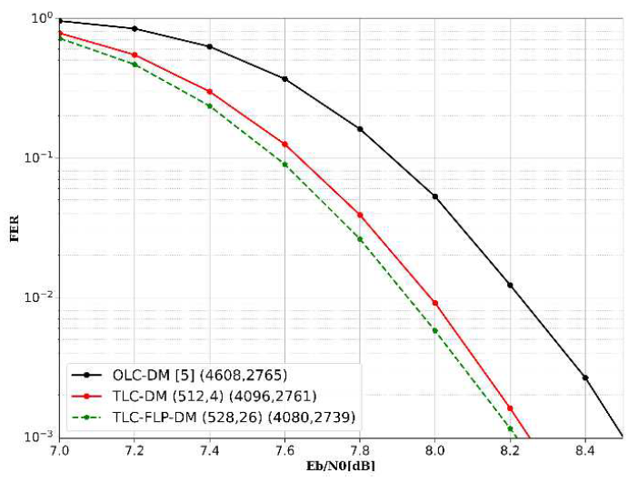 Fig. 6 shows the overall FER performance for N = 1024, n = 8, k = 4, M = 4 and R = 0.5. OLC-DM uses (2816, 1408) LDPC codes, TLC-DM uses (768, 32) and (2048, 1376) LDPC codes and TLC-FLP-DM uses (788, 50) and (2028, 1358) LDPC codes. In the case where n = 8 and k = 4, 64 patterns are employed. This means that for OLC-DM, the LLR values for the symbol bits must be calculated by considering all 64 patterns, whereas TLC-DM only needs to consider the single pattern estimated from the first layer. In terms of performance, TLC-DM exhibits greater gains compared to OLC-DM. Furthermore, TLC-FLP-DM performs a 20-bit transfer from the second codeword, which enables [TeX:] $$R_1$$ to be set more optimally without significantly altering [TeX:] $$R_2$$ Overall, FLP yields a modest improvement in performance. Ⅴ. ConclusionIn this paper, we proposed a TLC-DM-OFDM-IM scheme in which data for DM-OFDM-IM is separately encoded into first and second layer codewords, followed by SCD at the receiver. The proposed approach leverages decoded first layer during the second layer decoding process, providing accurate index bit estimates and significantly reducing frame errors in the second layer. We also provided a theoretical explanation of the advantage of the TLC scheme in terms of achievable rate through a capacity analysis of TLC-DM-OFDM-IM. Furthermore, to expand the range of feasible code rate configurations, we introduced a FLP scheme, in which the first layer is composed of the first codeword and a portion of the second codeword, while the second layer consists of the remaining part of the second codeword, allowing more flexible rate assignments for each codeword. In addition, SCD simplifies symbol bit LLR computations, substantially reducing decoding complexity. Simulation results demonstrated that the proposed TLC-FLP-DM-OFDM-IM achieves lower FER compared to conventional DM-OFDM-IM, clearly illustrating the benefits of combining TLC, SCD, and FLP in DM-OFDM-IM systems. BiographyBiographyKezhong JinFeb. 2001: B.S. degree, Zhe- jiang University of Techno- logy Feb. 2004:M.S. degree, Zhe- jiang University of Techno- logy Aug. 2023:Ph.D. degree, Chon- nam National University [Research Interests] machine learning, multiobjective evolutionary algorithm, resource allocation opti- mization in wireless networks [ORCID:0000-0002-0796-2662] BiographyHosung ParkFeb. 2007: B.S. degree, Seoul National University Feb. 2009: M.S. degree, Seoul National University Mar. 2013:Ph.D. degree, Seoul National University [Research Interests] channel codes for communi- cations systems, coding for memory/storage, coding for distributed storage, communication signal processing, compressed sensing, network information theory [ORCID:0000-0001-7854-7792] References
|
StatisticsCite this articleIEEE StyleS. Choi, K. Jin, H. Park, "Two-Layer Coding with Flexible Layer-Partitioning for Dual-Mode OFDM-IM," The Journal of Korean Institute of Communications and Information Sciences, vol. 50, no. 11, pp. 1700-1708, 2025. DOI: 10.7840/kics.2025.50.11.1700.
ACM Style Seung-gi Choi, Kezhong Jin, and Hosung Park. 2025. Two-Layer Coding with Flexible Layer-Partitioning for Dual-Mode OFDM-IM. The Journal of Korean Institute of Communications and Information Sciences, 50, 11, (2025), 1700-1708. DOI: 10.7840/kics.2025.50.11.1700.
KICS Style Seung-gi Choi, Kezhong Jin, Hosung Park, "Two-Layer Coding with Flexible Layer-Partitioning for Dual-Mode OFDM-IM," The Journal of Korean Institute of Communications and Information Sciences, vol. 50, no. 11, pp. 1700-1708, 11. 2025. (https://doi.org/10.7840/kics.2025.50.11.1700)
|