One-Shot Deep Learning-Based Camera– LiDAR Extrinsic Calibration with Pyramid Dilation-Based Encoder

Ⅰ. Introduction

In recent years, sensor fusion technology has gained significant attention as research in drones and autonomous driving continues to advance rapidly. These applications operate in highly complex and dynamic environments, where relying on a single sensor typically proves insufficient for robust perception. By combining the strengths of different sensing modalities, detection accuracy can be considerably improved, and the number of false positives can be reduced^[1].

Previous studies have demonstrated that no single sensor can consistently provide precise recognition under all conditions. Cameras may struggle under low-light or adverse weather conditions, whereas light detection and ranging (LiDAR) and radar have their limitations, such as occlusions or difficulties in detecting certain materials. Sensor fusion addresses these challenges by combining complementary information from different modalities, thereby improving understanding, object detection, and decision-making capabilities for autonomous systems.

Integrating data from cameras and LiDAR can yield significant benefits. Cameras capture a rich array of visual details, including color, contrast, and texture, which are essential for accurately identifying and classifying objects within a scene. Their high-resolution contributes to a better understanding of the context and subtle features, thereby facilitating complex scene analyses necessary for tasks such as object detection and semantic segmentation.

In contrast, LiDAR excels at providing precise depth measurements and accurate distance information that cameras alone cannot offer. Its ability to generate detailed three-dimensional (3D) spatial data makes it ideal for developing accurate models of environments, detecting obstacles, and discerning spatial geometries. Moreover, LiDAR maintains consistent performance regardless of the lighting conditions, ensuring reliable detection even when visual cues are less effective.

When these two sensor types are combined, their complementary strengths lead to a better comprehensive understanding of the environment. When the detailed visual information from cameras is aligned with the precise spatial measurements of LiDAR, the limitations inherent to each sensor when used independently can be effectively addressed.

Ultimately, leveraging sensor fusion harnesses the unique advantages of cameras and LiDAR to construct a more robust and reliable perception system. This integrated approach not only enhances object detection and situational awareness but also significantly improves overall system resilience, which makes it a crucial strategy for advancing autonomous driving and drone navigation technologies.

Conventional calibration techniques rely on artificial markers such as checkerboards^[2-4] and specialized calibration targets^[5] to compare LiDAR 3D points against predetermined patterns (for example, a chessboard) to estimate extrinsic parameters and calibrate both LiDAR and camera systems. This early calibration approach also involves matching feature points between LiDAR point clouds and camera images to determine the relative transformation between the two sensors. However, these marker-based methods are typically time-consuming and labor-intensive and typically require offline processing, which renders them impractical for real-time applications in drone or autonomous driving environments.

In dynamic scenarios, such as robot operations, sensor positions may shift slightly over time, leading to accumulated drift that requires frequent recalibration. This limitation of conventional methods has spurred the search for more adaptive solutions. Deep learning (DL) has emerged as a promising alternative for extrinsic calibration. By leveraging its ability to automatically learn robust feature representations and estimate sensor transformations in real time, DL can streamline the calibration process, reduce manual intervention, and maintain accuracy under continuously changing conditions.

In this study, we propose an online novel method for calibrating the extrinsic parameters between a single camera and a single LiDAR sensor. Unlike conventional approaches, the proposed model does not rely on predefined patterns or calibration objects. Our key contributions can be summarized as follows:

The overall network comprises three parts: a self-developed feature extraction network using a novel pyramid-like dilation-based encoder with a channel attention module for both RGB and depth images; a feature matching layer; a global feature aggregation network.

The proposed model can be categorized as a lightweight model with only approximately 10 million parameters, which is significantly smaller than the number of parameters of existing methods.

Ⅱ. Related Research

According to the calibration targets, previous research on extrinsic calibration has largely focused on three main categories: target-based, target-less, and learning-based methods, each offering distinct approaches and benefits.

First, target-based extrinsic calibration methods rely on objects with certain shapes or structures as targets to capture correspondences between a camera and LiDAR. Grammatikopoulos et al.^[6] proposed a target-based calibration scheme using planar targets consisting of an AprilTag marker and a custom retroreflective target to perform both spatial and temporal LiDAR calibration. In this scheme, AprilTag is employed to capture two-dimensional (2D) points from a camera, whereas retroreflective is employed to capture 3D points from LiDAR. In addition, Agrawal et al.^[7] introduced a custom retroreflective calibration target comprising a trihedral corner in the center of a square with a reflective surface.

Second, target-less methods eliminate the requirement for predefined targets by autonomously estimating extrinsic parameters based on meaningful information from the surrounding environment. Bai et al.^[8] proposed a calibration method that leverages line features for aligning the extrinsic parameters of camera and LiDAR sensors based on the observation that line features are prevalent in most environments. Ou et al.^[9] proposed a target-less calibration scheme that involves extracting key points from camera images through visual simultaneous localization and mapping and performing hand-eye calibration to estimate the extrinsic parameters of the system.

Finally, learning-based approaches use end-to-end DL models, eliminating the need for manually defined features. These methods leverage neural networks to automatically extract valuable information, thereby streamlining and improving the calibration process. The learning-based method RegNet was first introduced by Schneider et al.^[10]. RegNet involves two branches of convolutional neural network (CNN)-based feature extraction, which is a CNN-based feature that matches several fully connected layers to regress the calibration parameters. The RegNet architecture has become the basic structure for building DL models for LiDAR–camera extrinsic parameter calibration. CalibDNN^[11] has a similar architecture to RegNet but performs calibration in a single iteration. CALNet^[12] is also based on the RegNet architecture with an optimized feature matching that employs spatial pyramid pooling. CalibRCNN^[13] uses a recurrent network, such as long short-term memory, for feature matching, which allows the extraction of both spatial and temporal features. PSNet^[14] improves RegNet by introducing parallel subnetworks in the feature extraction process, thereby enhancing feature extraction by using multiresolution feature maps.

Unlike these methods, our approach prioritizes the creation of a DL model specifically for practical, real-world deployment. To accomplish this, we develop a lightweight model that ensures efficiency and real-time usability for calibrating extrinsic parameters.

Ⅲ. Proposed Methods

In this work, a deep neural network architecture for estimating the extrinsic calibration parameters between LiDAR and camera sensors is proposed. The proposed network integrates a pyramidal dilation convolution block for feature extraction based on depth and RGB images. Different from existing methods, which primarily focus only on performance, the proposed model uses few model parameters, only 10 million parameters, for prediction, making it lightweight and well-suited for real-world applications.

3.1 Data Preprocessing

The initial extrinsic parameters in the form of matrix obtained from the datasets used in this study, referred to as T_init, which include both the rotation parameters (R_init) and translation parameters (t_init), enable the transformation of point cloud data from their original coordinate system to the appropriate camera coordinate system. This is achieved using the following transformation equation:

Once the point cloud data have been converted into the camera coordinate system, the intrinsic parameters of the camera, including the focal length, can be used to project the point cloud data onto the image plane using the pinhole camera model. In this process, each X and Y value from 3D point P_i = (X_i, Y_i, Z_i) is used to map the location of each point cloud data to a corresponding point p_i = (u_i, v_i) on the 2D image plane and use the Z data to determine the depth of each point in the 2D image plane. The resulting depth images are created by assigning the inverse depth of each point as the pixel value for the corresponding location on the depth image. This projection process can be mathematically represented as follows:

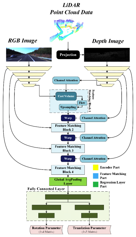
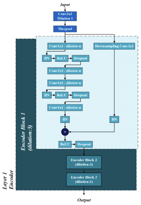
Here, d_i denotes the depth of the LiDAR point cloud data following its projection onto the image plane. This depth information is used to create a depth map that corresponds to the associated RGB image data. K represents the intrinsic parameters of the camera sensor.

Fig. 1.

Overall proposed model architecture.

3.2 Network Architecture

The proposed calibration network can be divided into three primary parts: two feature extraction branches (for depth and RGB images), a feature matching layer, and a regression layer which can be seen in Figure 1. The structure and function of each component are described in detail in this section.

The feature extraction network is divided into two branches for extracting features from the original RGB images and the depth images generated from the point cloud data projection. The network comprises a pyramid dilation convolution block. Inspired by Liang^[15], the proposed convolution block comprises multiple convolution layers with varying dilation rates, arranged from large to small in a pyramid-like structure like shown in Figure 2. The proposed feature extraction network also involves four feature extraction steps, each of which is used as input in the next step of the feature extraction network.

Fig. 2.

Pyramid Dilation Encoder Block.

By employing this novel feature extraction design, the efficiency of feature extraction is enhanced, allowing the proposed model to capture broader contextual information rather than focusing solely on individual pixels. As a result, we can reduce the number of layers within the feature extraction module without compromising the model's performance, leading to a lightweight yet effective AI model.

The feature matching layer, inspired by LCCNet^[16], compares the feature maps obtained from both feature extraction branches (RGB and depth images) in the feature extraction network by calculating the 3D correlation volume of the corresponding pixels in the RGB and depth feature maps that represent the spatial correlation between both data. This correlation layer can be expressed as follows:

where x(p_i) denotes the feature of RGB images or depth maps at the i^th or j^th position in the corresponding feature map and D represents the set of points in a square area, which is the feature map area in this context. Based on the 3D correlation volume, the optical flow between the two feature sets can be estimated. This estimation is performed by a learning-based layer, where a standard convolutional layer produces a two-channel output representing the horizontal and vertical flow vectors. In this layer, a lightweight channel attention mechanism is incorporated, which uses the features extracted from the depth image data. This mechanism transforms the input features into query, key, and value representations via a single linear layer, resulting in three distinct tensors. These three tensors are then processed via some layers, allowing the model to adaptively highlight significant channels. This streamlined attention mechanism enhances the representation of relevant channel features while diminishing the influence of less informative features.

The regression layer takes features from the final layer of the feature matching module as input. It comprises multiple stacked convolutional layers and incorporates an average pooling layer to reduce the feature size while preserving the essential information. The pooled features are then passed through a global fully connected layer, followed by two separate branches: one for estimating rotation in 1 × 4 quaternion format rotation matrix and the other for predicting the 1 × 3 translation vector.

3.3 Loss Functions

In this study, the Euclidean distance loss is used as the translation loss (LT). The Euclidean distance loss is defined as follows:

The quaternion representation is used as the rotation loss (LR) because it effectively captures directional information. Measuring this type of information using the Euclidean distance would be inaccurate; thus, the quaternion angular distance is employed. The quaternion angular distance is defined as follows:

In addition to the regression loss, the loss function incorporates the point cloud distance. This is computed by applying the predicted transformation matrix to the point cloud, calculating the distance for each batch sample, and using the initial transformation matrix within the L2 normalization equation. The result is then averaged over the entire dataset. The point cloud loss is defined as follows:

Based on these three loss functions, a translation loss (Ltotal), a rotation loss (LR), and a point cloud distance loss (LP) are each weighted and then summed as follows:

where λ_T, λ_R, and λ_P denote the loss weights for L_T, L_R, and L_P, respectively.

3.4 Calibration Inference

The proposed network does not directly estimate the extrinsic calibration matrix. However, the depth image is generated based on a randomly applied miscalibration transformation matrix; thus, the predicted output represents the deviation from the initial parameters, which is an error matrix applied to the original transformation. Consequently, the extrinsic calibration matrix is obtained as follows:

Recent learning-based methods for extrinsic calibration primarily rely on iterative inference approaches that use multiple networks across different ranges to progressively refine the calibration. In contrast, this study employs a one-shot approach that uses a single network for direct estimation.

Ⅳ. Experiment

4.1 Dataset

The experiment is conducted using the KITTI-Odometry dataset, which comprises 22 sequences that are split into two parts: sequence 01 until 21 are used as training data with approximately 39011 frames, and sequence 0 is used as validation and testing data with approximately 4541 frames. The dataset contains data obtained using two regular cameras, two grayscale cameras, and several other sensors. In our experiment, we use RGB images from camera 0.

We also use the point cloud data from Velodyne HDL-64E LiDAR provided in the KITTI-Odometry dataset for generating depth maps. This dataset already includes synchronized RGB images and LiDAR point clouds, which ensure precise alignment between visual and depth information.

This synchronization eliminates the need for additional processing to align the two data types, allowing for more accurate depth map generation and more reliable integration of camera and LiDAR data in our extrinsic calibration task.

To simulate misalignment in the LiDAR–camera system, the extrinsic parameters are varied within a range of 0.25m-10.0°, mimicking real-world sensor inaccuracies and misalignments.

4.2 Training Details

The proposed DL model is implemented using the PyTorch library and trained on an NVIDIA Titan XP GPU, paired with an Intel Xeon Silver 4215R CPU and 32GB of RAM. The proposed model consists of approximately 10M parameters. Training is performed using a batch size of 16 over 200 epochs. The initial learning rate is set to 1e^-4 and is reduced by a factor of 0.3 whenever the validation performance stagnates for 10 consecutive evaluations. The Adam optimizer is also used to update model weights during training.

4.3 Results and Discussion

The performance results of the proposed method are presented in Table 1. This result is obtained by applying a one-shot approach to camera–LiDAR extrinsic calibration estimation with a maximum error range of 0.25 m for translation and 10° for rotation. The proposed estimation model is lightweight and ensures stable real-time performance without decreasing the quality of the estimation. The performance of the proposed method is then compared to several existing methods shown in Table 2.

The performance results shown in Table 1 are evaluated by measuring the rotation and translation errors of the predicted extrinsic parameters. For translation errors, we employ absolute errors from the Euclidean distance between the predicted and ground truth translation vectors. In addition, for rotation errors, we employ absolute errors from the Euler angle difference, which are the roll, pitch, and yaw between the predicted and ground truth rotations.

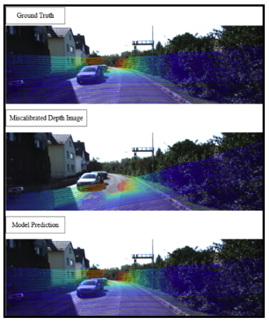
To assess the effectiveness of the proposed method, we present a performance comparison in Table 2, focusing on the translation and rotation errors. All existing methods are evaluated under the same misalignment conditions as the proposed model (0.25 m and 10°). Figure 3 presents the visual results, displaying the misaligned input, the calibrated image, and the ground truth. The results demonstrate that the proposed method effectively aligns the point cloud to restore its original position and orientation, as shown in the ground truth.

Fig. 3.

Prediction results sample visualization.

The results demonstrate that the proposed method outperforms existing approaches in all translation error metrics. While it does not achieve the highest accuracy in rotation error metrics, its performance remains competitive. Importantly, this level of accuracy is attained despite a substantial reduction in number of model parameters. Specifically, the proposed model utilizes approximately 10 million parameters, compared to the 13.5 million parameters used in parts of the feature extraction branches of PSNet^[14], CalibRCNN^[13], CalibDNN^[11], and CALNet^[12], which rely on ResNet-18 encoders with over 10 million parameters. As shown in Table 3, these findings indicate that the proposed method achieves high translation accuracy with a significantly reducedparameter count. Nevertheless, although its rotationaccuracy is on par with existing methods, further improvements are still possible.

Moreover, in terms of real-time performance analysis, as presented in Table 4, it was conducted within the training environment described at the beginning of Chapter 4. The proposed model processes each frame of both RGB and depth image data in approximately 59 milliseconds, demonstrating its suitability for real-time applications. Furthermore, the GPU memory usage during inference is limited to 38 MB, and the storage requirement for the model’s weights is 112 MB. These characteristics support the feasibility of deploying the proposed model on edge devices.

Ⅴ. Conclusion

This study proposes a DL-based model for camera –LiDAR extrinsic calibration. The proposed model introduces a novel feature extraction strategy that uses a pyramid-like dilation-based convolution layer combined with a channel attention module at each extraction level.

The proposed method calibrates extrinsic parameters under initial misalignments of up to 0.25 m in translation and 10.0° in rotation. The proposed model achieves mean translation errors of 0.0102, 0.015, and 0.005 m along the X, Y, and Z axes, respectively, and mean rotation errors of 0.41°, 0.36°, and 0.18° for roll, pitch, and yaw, respectively.

Although the current dataset encompasses a range of real-world driving scenarios, future work will aim to extend the applicability of the proposed deep learning-based extrinsic calibration method to more challenging conditions, such as rain, snow, and fog. This will be achieved by incorporating datasets that specifically represent these adverse environments. Furthermore, future research may not only focus on enhancing model performance but also explore novel approaches to training the AI model itself.